One question I’ve been asked a large number of times is how to perform a power calculation in Mendelian randomization for a binary exposure. We wrote a longer paper on the difficulties of MR with a binary exposure previously (Mendelian randomization with a binary exposure variable: interpretation and presentation of causal estimates), but we removed details on power calculation due to limited word count.
The short answer is that it's not simple, and potentially not possible unless you have additional data. If the gene—exposure associations are estimated on the odds ratio scale, it makes a big difference to power if the exposure is rare (e.g. for an odds ratio of 1.2, the genetic variant would increase exposure prevalence from 0.1% to 0.12% in absolute terms) or the exposure is common (e.g. the genetic variant increases exposure prevalence from 10% to 12%). Power depends on the absolute magnitude of the increase in the exposure prevalence, not the relative increase on the odds ratio scale. So if you have no way of estimating genetic associations with the exposure on an absolute scale (such as linear regression of the exposure on the genetic variant), then you can't calculate power.
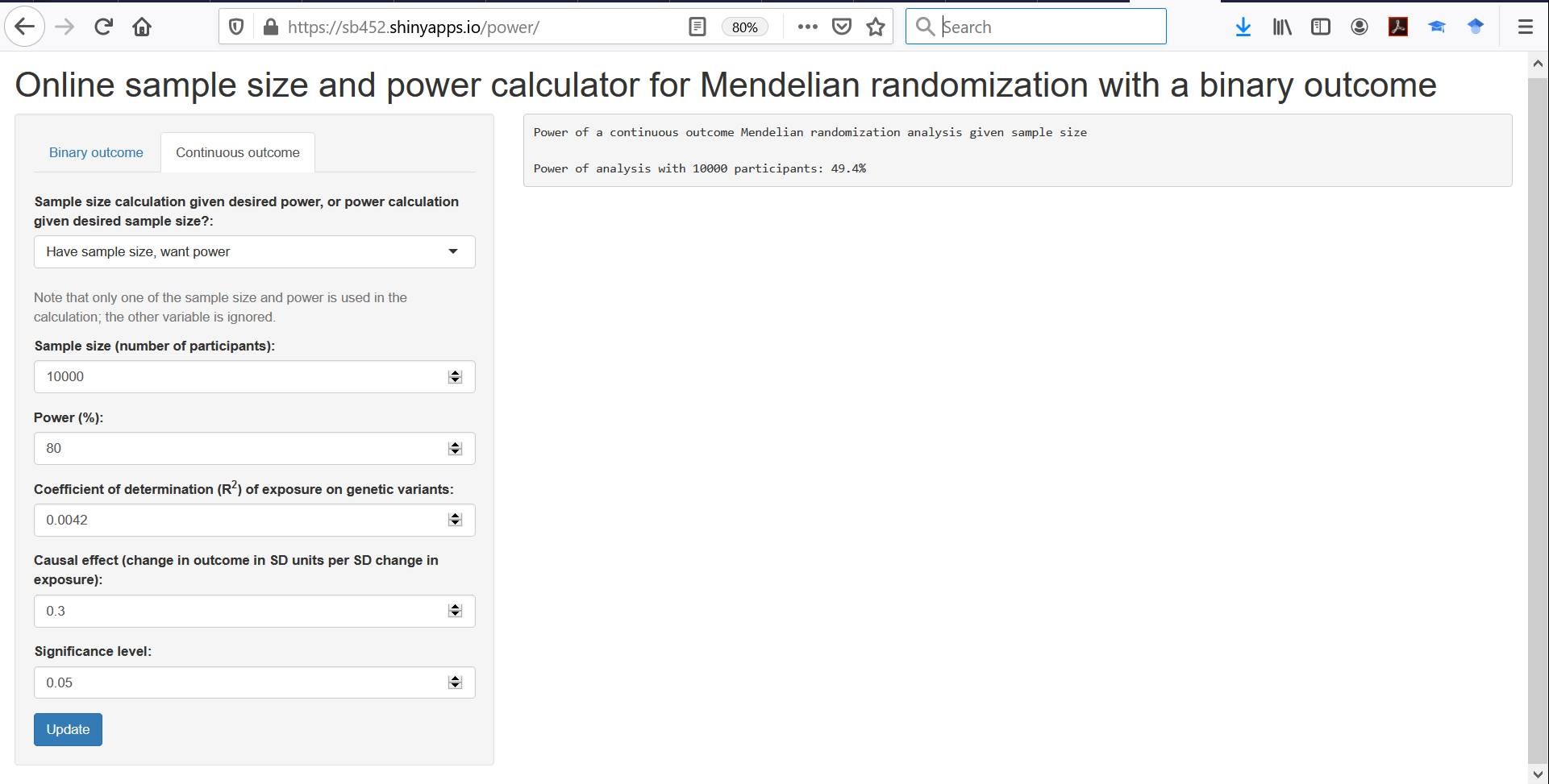
If you can get the IV—exposure associations on an absolute scale (e.g. the genetic variant increases the prevalence of the outcome by 2% - say from 10% to 12%), then you can calculate power. But power calculations are still not simple as power is normally given for a proposed effect size per 1-SD unit increase in the exposure, and a 1-SD change for a binary exposure may be a little difficult to conceptualize. Instead, we can consider the proposed per 1 unit increase in the exposure (from 0 to 1). In this case, you can use standard tools for power calculation (such as Online sample size and power calculator for Mendelian randomization with a binary outcome), but instead of the R^2 measure, you need a different value. This is obtained by taking the beta-coefficient from linear regression of the exposure on the genetic variant (call this number beta). For a biallelic SNP, instead of the R^2 statistic, you want beta^2*2*MAF*(1-MAF).
So if you have a genetic variant that is a SNP with a minor allele frequency of 0.3 that increases the prevalence of the exposure by 10%, then your replacement “R^2 value” is 0.1^2*2*0.3*0.7 = 0.0042. Power to detect a 0.3 SD increase in the outcome per 1 unit increase in the exposure in a sample size of 10,000 would be around 50%, as shown in the screenshot below:
A quick simulation exercise demonstrates that this value is fairly accurate:
set.seed(496)
times = 1000
parts = 10000
pval = NULL
for (j in 1:times) {
g = rbinom(parts, 2, 0.3)
x = rbinom(parts, 1, 0.2+0.1*g)
y = rnorm(parts, 0.3*x)
pval[j] = summary(lm(y~g))$coef[2,4]
}
sum(pval<0.05)
> [1] 492
Hope that is helpful!